

Every winter, a handful of hours decide how expensive a utility’s balance gets. It turns cold faster than last week’s data suggests, the sun sets before the evening peak, and on a calm day there is little wind to fill the gap. This winter adds pressure: EU gas storage ended October about 15 percentage points below its five-year average, German year-ahead power trades around 80% above a year ago, and October day-ahead prices in Germany were more than double last October’s. A forecast miss in the wrong hour costs more than usual.
In our recent webinar with LCP Delta, we showed how we forecast residential solar and consumption at Podero, how those forecasts become trades, and why steering the devices themselves keeps imbalance low. Our guest, Shivam Malhotra, Head of Power Trading at LCP Delta, explained how a more wind-driven system is changing forecasting, with Great Britain as a case study. Here are the main points.
Key takeaways
- In winter, a few cold, calm evening hours drive most of the imbalance risk for utilities with heat pumps, solar and EVs in their portfolio.
- Blending several weather models and correcting them with live production data lowered Podero’s day-ahead solar forecast error from 8.7% to 8.4% of panel capacity, and to 7.7% two hours ahead.
- A forecast miss is paid for in the hour it happens: on 6 August 2026, the Austrian imbalance price peaked at €8,906/MWh.
- When flexible devices are steered to the same curve that is traded, imbalance becomes something a utility can measure and reduce device by device.
- In Great Britain, more wind and grid constraints make forecasting harder, and NESO projects constraint costs of around £7bn by 2030.
Three ways winter drives up imbalance costs
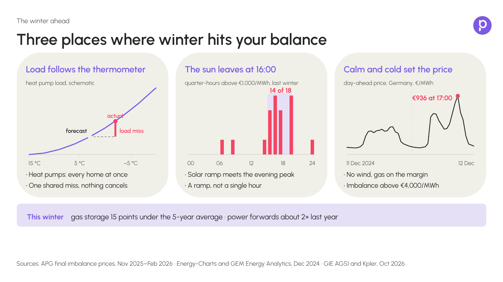
First, it gets cold fast. Heat pump load follows the thermometer, and every home reacts at the same moment. A forecast built on the last two weeks struggles when tomorrow is suddenly much colder, which is why the transition months in autumn and spring produce so many misses. Because all heat pumps miss in the same direction, the errors add up instead of cancelling out.
Second, the sun sets before the evening peak. In December it sets around 16:00 in much of Central Europe, so solar output disappears just as households come home. The ramp from afternoon into evening is where the most expensive quarter-hours tend to sit.
Third, cold and calm set the price. When low temperatures meet low wind, gas plants are on the margin. On 12 December 2024, a cold and windless spell pushed the German day-ahead price to €936/MWh for the hour from 17:00.
How we forecast residential solar: let the weather models compete
Solar is mostly a physics problem. With a forecast of irradiance, temperature and wind speed, you can model what a PV system will produce. The catch with residential solar is that no two roofs are alike. Each home has its own tilt, orientation and shading, unlike a utility-scale plant with a known layout.
At Podero we start from several numerical weather prediction models from national weather services, plus a specialised provider that works from satellite imagery. Each has its own grid, starting conditions and strengths. Think of neighbours arguing about tomorrow’s weather, each with a different app: sometimes one is right, sometimes the other.
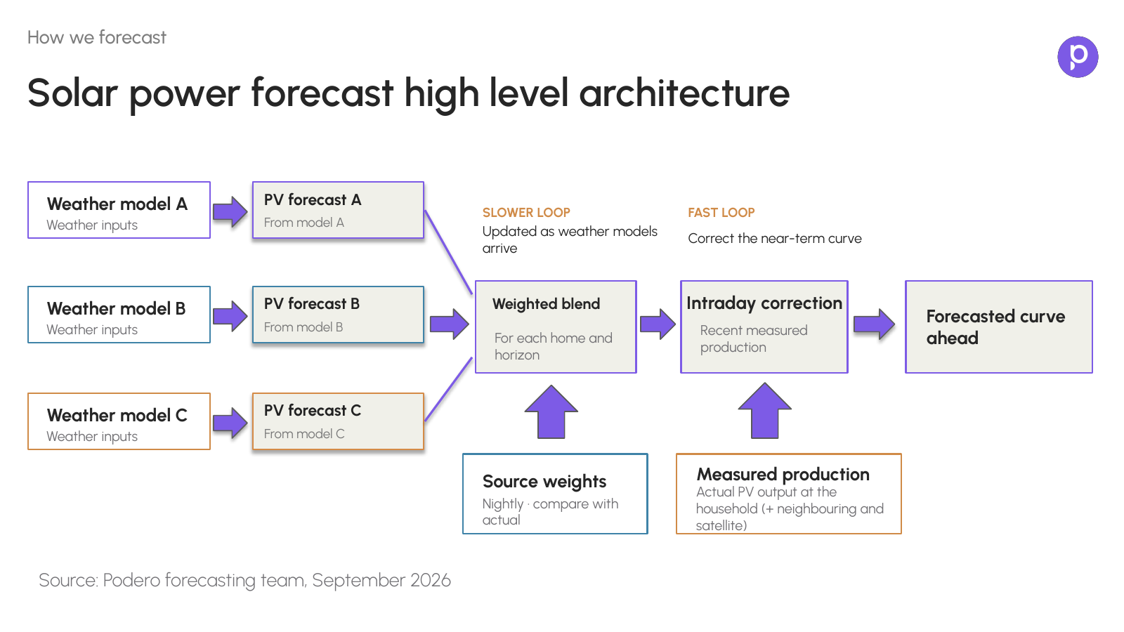
So we let the models compete, and we keep score. Every night we compare each model’s forecasts with what the panels actually produced over the past week, and we set each model’s weight for the days ahead. Because we connect directly to inverters, we see real production for every home, not only the meter reading. That is what makes the scoring work at household level.
On top of this slower loop runs a fast one. A lighter model uses the latest measured production to correct the next few hours, refreshed every 15 minutes. Today it uses each home’s own readings; next, we want to add neighbouring homes and satellite imagery.
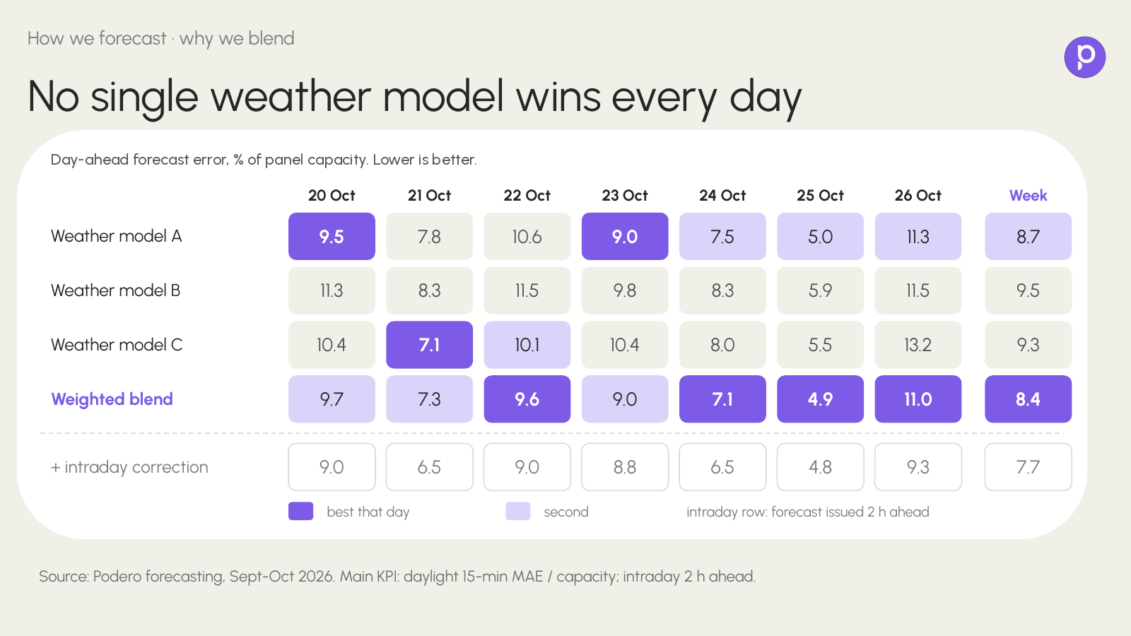
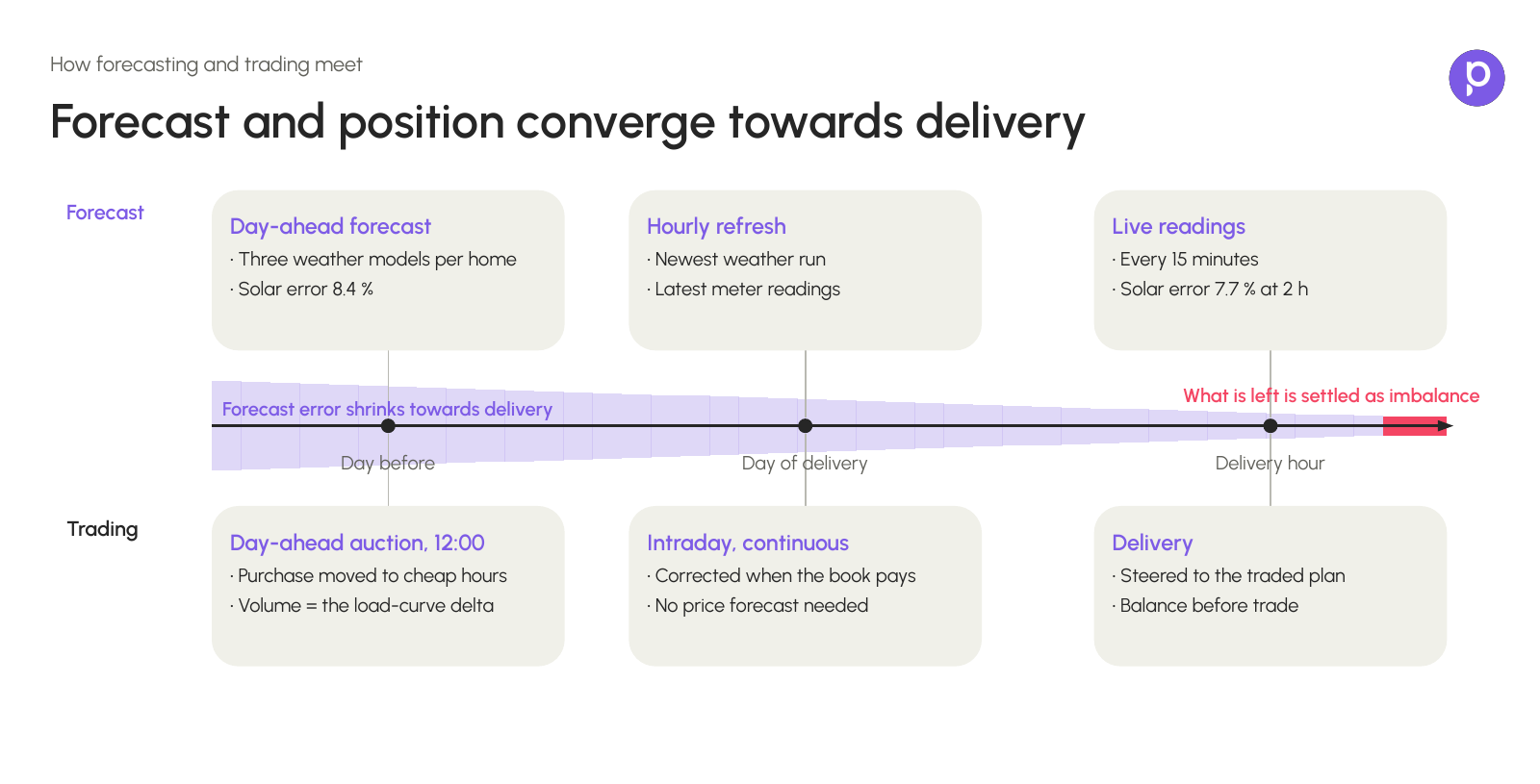
The effect shows in the numbers. Measured over September and October, the day-ahead error of the best single weather model was 8.7% of panel capacity. The weighted blend brought it to 8.4%, and the intraday correction, two hours ahead, to 7.7%. Just as important, no single model wins every day, which is exactly why we blend them.
Forecasting household electricity consumption: a human problem
Consumption is a different kind of forecast. It depends on people: when they come home, cook, run the dishwasher or plug in the car. A family baking for a birthday party will never show up in last week’s data.
At Podero we split each home’s load into parts before we forecast it. There is a base load of always-on and small appliances, and there are recognisable loads such as EV charging, heat pumps, dishwashers and ovens, each with its own signature of step size, duration and time of day. The model learns from recent history, detected load events and context such as weekday, holidays and the weather. It refreshes a curve for every home each hour, in 15-minute slots, two days ahead.
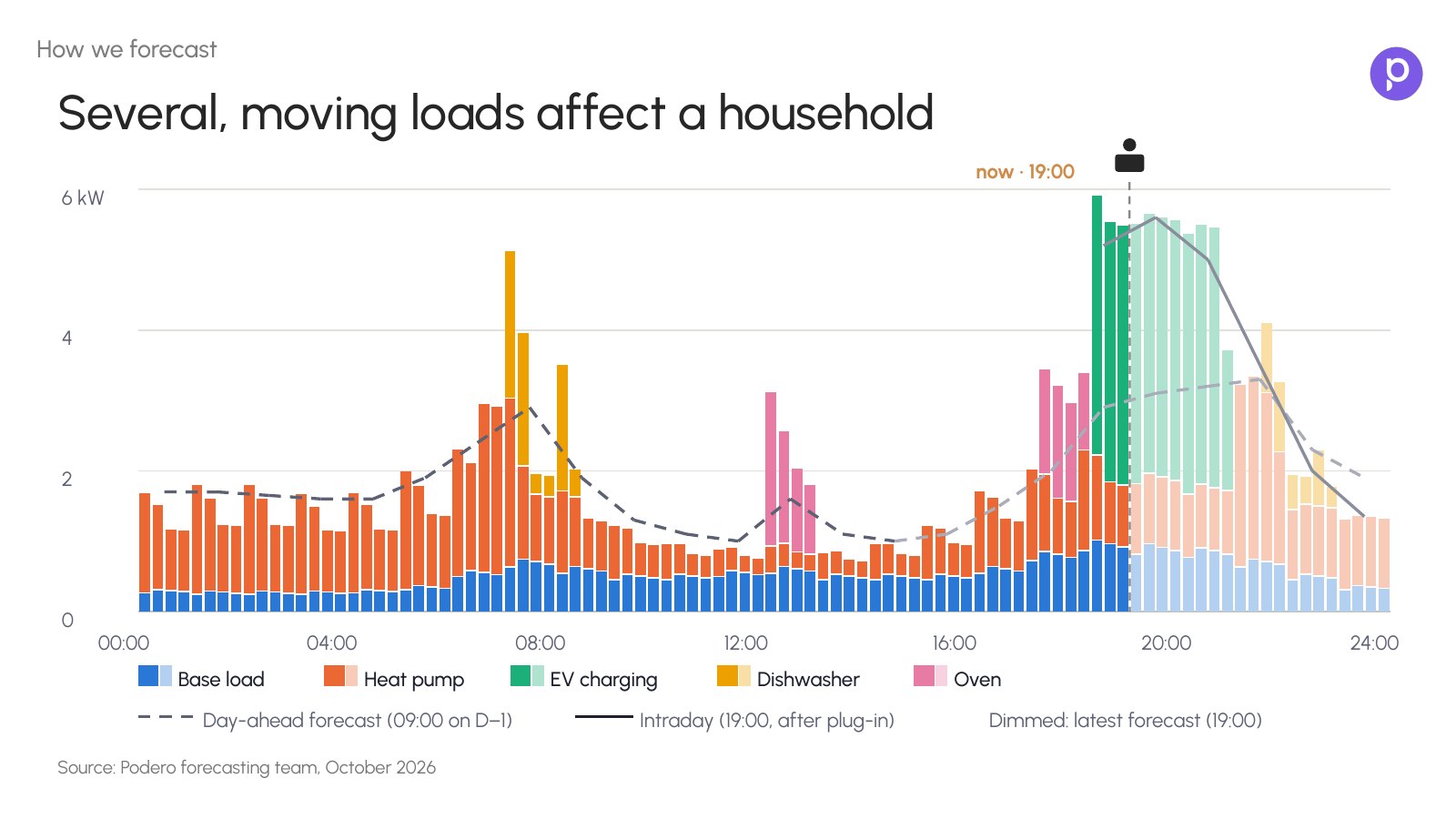
EV charging gets its own treatment, because it is the hardest part to predict. We forecast it in layers: the probability that a car plugs in during a given slot, how long it will charge if it does, and the base curve underneath. Once the car is actually plugged in, the intraday forecast updates straight away, because we then know roughly how long the charge will run.
No single home is fully predictable. Across a fleet, and with device-level data instead of one meter curve, the forecast becomes far more reliable than looking at a balance group’s load as a whole.
Why the hour decides what a forecast miss costs
If you trade in Austria, 6 August 2026 probably still hurts. For almost a full evening hour, the Austrian imbalance price stayed close to its peak of €8,906/MWh. The day-ahead price for that hour had been €229/MWh, and one hour later imbalance settled at €146/MWh again.
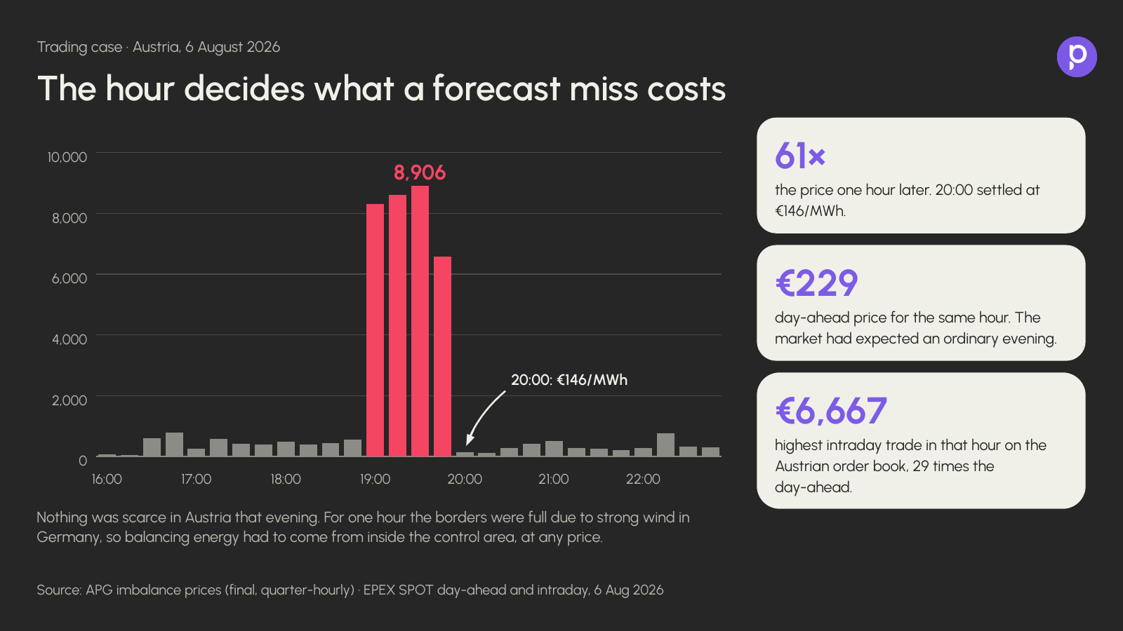
Nothing was scarce that evening. Strong wind in Germany filled the cross-border lines, so balancing energy had to come from inside the Austrian control area, at any price. The highest intraday trade in that hour reached €6,667/MWh, 29 times the day-ahead price. The lesson for forecasting is simple: a miss is not judged on its average size, but on the hour it lands in.
That is why forecasting and trading run as two lanes that meet at delivery. On the day before, we place residential flexibility in the day-ahead auction: consumption moves to cheap hours, export moves to expensive ones, and the traded volume is the change in the load curve. On the day of delivery we switch to the continuous intraday market. The forecast is refreshed every hour with the newest weather run and the latest meter readings, and we correct the position whenever the order book makes it worthwhile. Intraday trading needs no price forecast, because it works from the order book as it is.
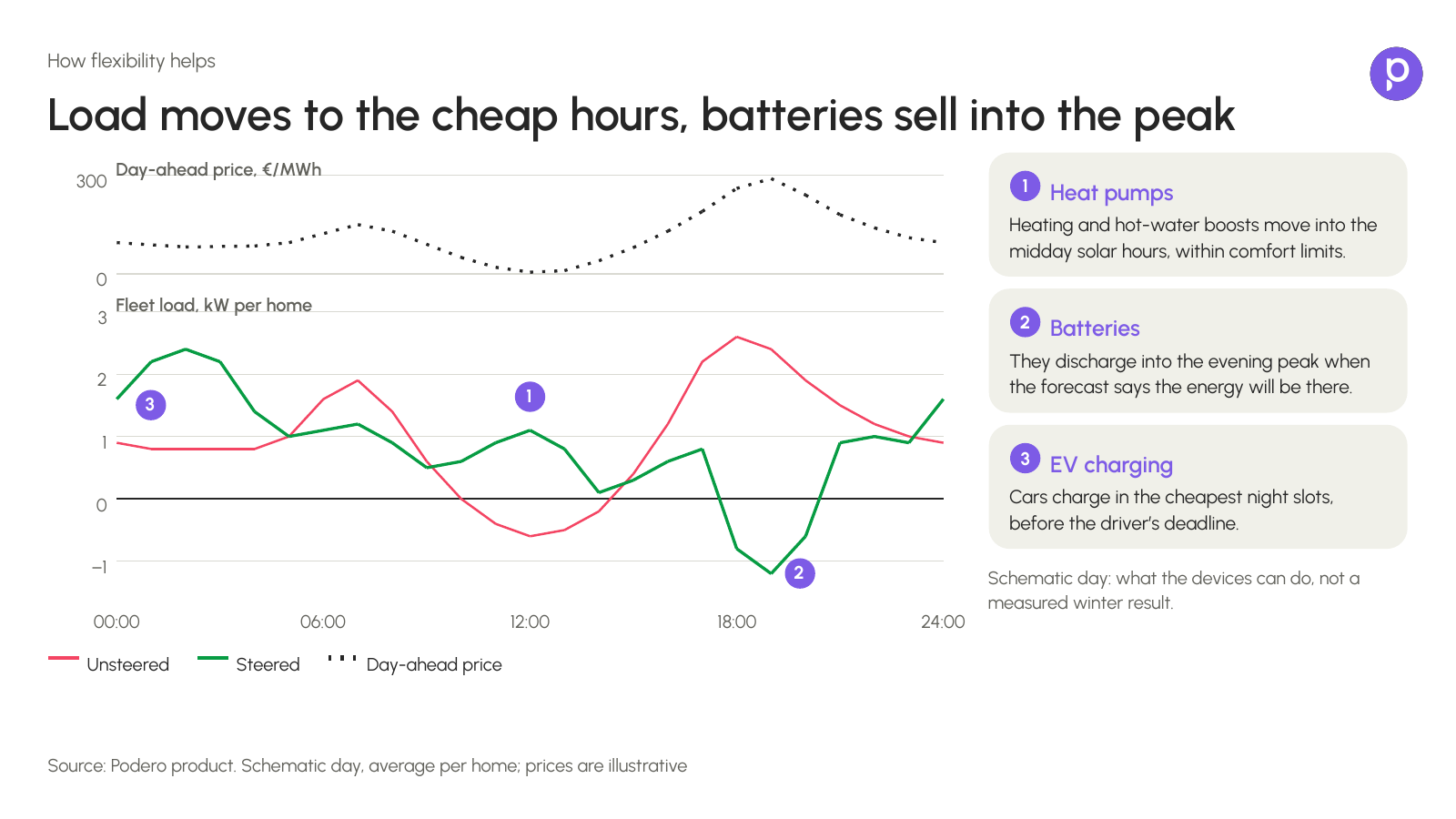
What the devices actually do follows from that plan. Heat pumps boost heating and hot water during the cheap midday solar hours, within comfort limits, so homes coast through the evening peak. Batteries discharge into the evening peak when the forecast says the energy will be there. Electric cars that plug in around 18:00 charge in the cheapest night slots instead, and are still full by morning.
How steering flexible devices keeps imbalance low
Put together, it is one loop. We forecast each home, plan a schedule for each device within its comfort limits, trade the resulting fleet curve day-ahead and intraday, steer every device to its own plan, and then measure what was delivered. The measurements go straight back into the next forecast.
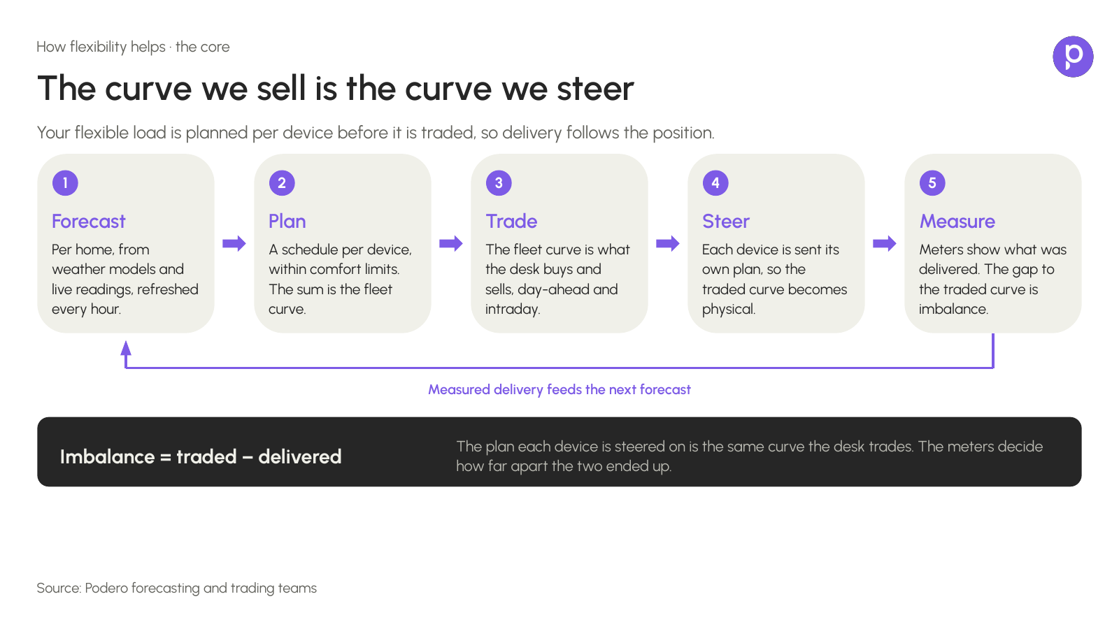
The key difference to a classic portfolio is control. Because we steer the devices, the flexible part of the load curve is something we actively shape, rather than only predict. Imbalance becomes simply the traded volume minus what was delivered, and it is measured per device, so utilities can see exactly how well the fleet followed the plan.
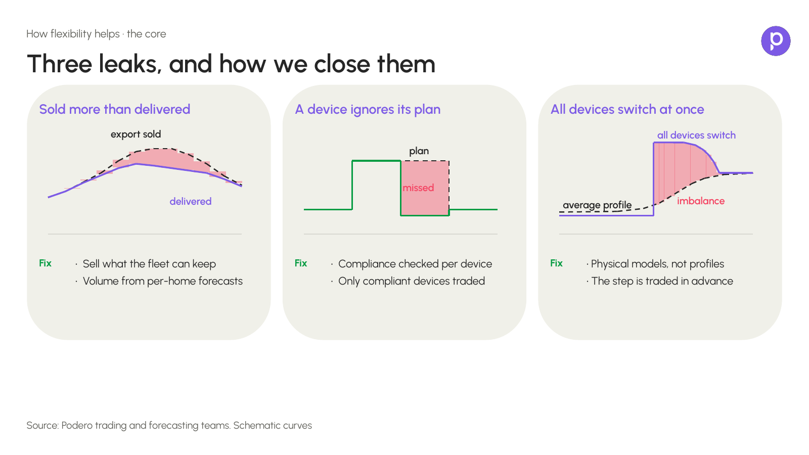
Three things can still open a gap between the two, and we design against each of them:
- Selling more than the fleet can deliver. Evening battery discharge is valuable, but those are also the hours with expensive imbalance. We set volumes from per-home forecasts and sell only what the fleet can keep.
- A device that does not follow its plan. We check compliance device by device, and only compliant devices are traded.
- Every device switching at once. Intraday opportunities are often a single 15- or 30-minute window, and a smooth forecast cannot show the sharp step when a whole fleet switches together. Physical models of each device capture that step, so it is traded in advance.
Wind, grid constraints and forecasting: lessons from GB
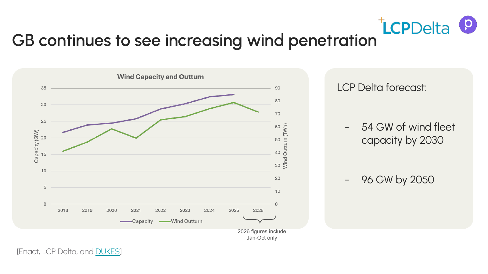
Wind complicates forecasting well beyond the residential side, and Great Britain shows where much of Europe is heading. UK wind farms generated a record 86.4 TWh in 2025, almost 30% of the country’s electricity, and wind output in the first nine months of 2026 was 14% above the previous record for that period. LCP Delta forecasts around 54 GW of GB wind capacity by 2030 and 96 GW by 2050, almost three times today’s level.
More wind means more complex forecasting. Output depends more on the weather, swings get bigger, and more of the imbalance appears at the last minute, so the horizon that matters moves from hours ahead to minutes ahead. GB is also a locationally constrained market: wind in Scotland often has to be turned down while gas plants in England are turned up. A useful forecast therefore has to say not only how much is generated, but where the need will be, and whether it shows up day-ahead, intraday or in last-minute balancing.
Extremes are a growing problem too. On 14 October 2026, according to LCP Delta, almost 8 GW of GB wind had to be curtailed because the power could not be transported, and the system saw its most negative net imbalance volume since 2020. GB balancing costs hit record levels in October.
“No forecast is going to be able to capture that, particularly if it’s a machine learning forecast, because it just hasn’t got that information in its training set.”
Shivam Malhotra, Head of Power Trading, LCP Delta
The cost of moving power around the grid shows up in the numbers. Constraint costs were about £1.8bn in 2025, 2026 is already higher than any previous year, and NESO has projected they could reach around £7bn by 2030 without further action. The National Audit Office puts the upper range at £7.8bn, and LCP Delta’s own modelling shows that network reforms could cut the 2030 figure substantially.
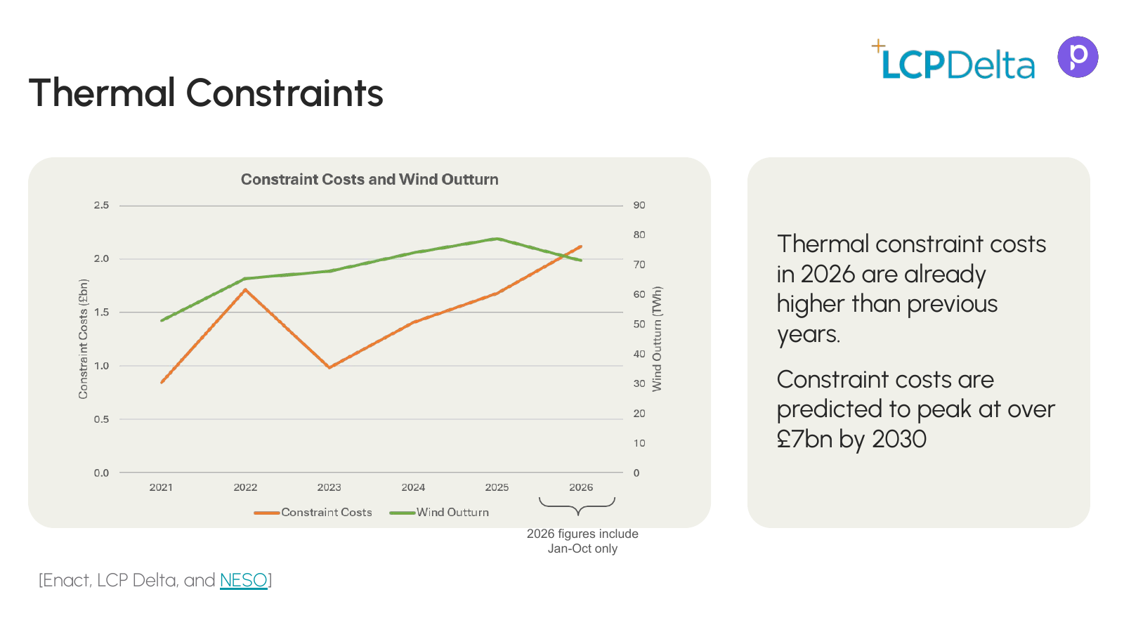
“We’ve already surpassed 2 billion pounds in constraint costs, and a lot of that is driven by wind generation and needing to turn up expensive gas. That’s obviously a problem, but it’s also an opportunity for flexibility to help solve some of these constraints.”
Shivam Malhotra, Head of Power Trading, LCP Delta
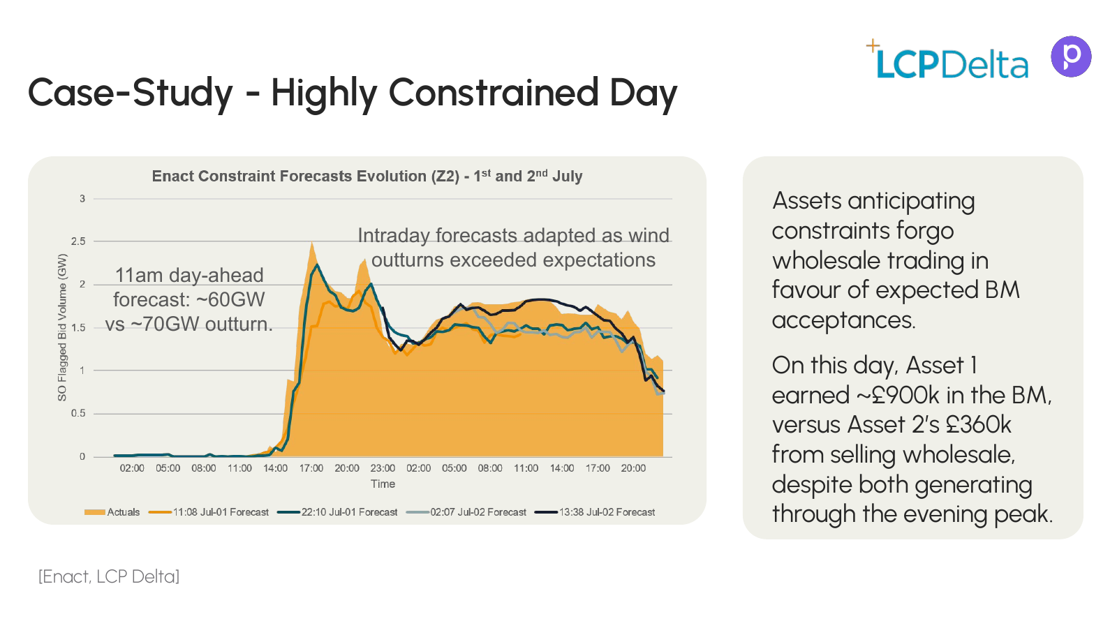
On a highly constrained day, the difference for flexible assets can be large. In one example from LCP Delta’s Enact data, an asset that anticipated the constraints and held back from wholesale trading earned around £900k in the Balancing Mechanism. A comparable asset that sold into the wholesale market earned about £360k, although both generated through the evening peak.
Not every market feels this equally. LCP Delta’s analysis shows the GB day-ahead market has been relatively unaffected, and more volatility does not automatically mean wider day-ahead spreads. Balancing, on the other hand, is getting harder, with imbalance volumes varying more from year to year. Demand-side measures such as the Demand Flexibility Service have helped, and better visibility of the generation that is actually available is what lets flexible assets decide when and where to act.
Getting ready for winter
Winter will test every forecast, and the expensive hours will come whether the forecast is ready or not. What makes the difference is how close the traded curve stays to what is delivered. With household flexibility, that gap can be designed small: forecast each home, plan each device, trade the fleet curve and steer devices to it.
Frequently asked questions
Why are imbalance costs higher in winter?
Three things come together. Heat pump load rises across all homes at once when it turns cold, so forecast errors add up instead of cancelling out. Solar output disappears around 16:00, just before the evening peak. And on cold, windless days, gas plants set the price. This winter, low gas storage and higher power prices add to the risk.
How does Podero forecast residential solar production?
We combine several numerical weather prediction models and weight them every night based on how well each matched the measured production of each home over the past week. A faster intraday model then corrects the next few hours with live production data every 15 minutes. In September and October 2026, this lowered the day-ahead error from 8.7% of panel capacity for the best single model to 8.4% for the blend, and to 7.7% two hours ahead.
Why is household electricity consumption hard to forecast?
Consumption depends on human behaviour: when people come home, cook or plug in their car. We split each home’s load into a base load and recognisable device loads, such as EV charging and heat pumps, and forecast EV charging separately as a probability of plug-in and charging duration. Across a fleet, and with device-level data, the forecast becomes far more reliable than a single balance group curve.
How does residential flexibility reduce imbalance costs?
The devices are steered to the same curve that is traded on the day-ahead and intraday markets. Each device gets its own plan, compliance is checked device by device, and physical models capture the sharp steps when many devices switch at once. Imbalance then becomes the measurable gap between what was traded and what was delivered.
How are grid constraints changing forecasting in Great Britain?
More wind makes output more weather-dependent and shifts imbalance towards the last minute, while transmission constraints mean wind is often turned down in Scotland and gas turned up in England. Constraint costs passed £2bn in 2026, and NESO has projected around £7bn by 2030. Flexible assets that anticipate constraints can earn more in the Balancing Mechanism than in the wholesale market.
Sources
- EU gas storage: Gas Infrastructure Europe AGSI data, via bne IntelliNews, 28 October 2026.
- German power prices: EEX year-ahead baseload, via Tacto, 26 October 2026; October day-ahead average, via Bloomberg / Energy Connects, November 2026.
- German day-ahead price, 12 December 2024: Bundesnetzagentur / SMARD.
- Austrian imbalance prices, 6 August 2026: Austrian Power Grid (APG) final quarter-hourly prices; EPEX SPOT day-ahead and intraday prices.
- Solar and household forecast results: Podero forecasting team, September to October 2026. Error is the mean absolute error as a share of panel capacity, on daylight 15-minute slots.
- UK wind generation: Department for Energy Security and Net Zero, via OilPrice.com; NESO data, via Bloomberg / Energy Connects, October 2026.
- GB wind capacity forecast, 14 October 2026 curtailment, day-ahead and imbalance analysis, constrained-day example: LCP Delta (Enact), presented in the webinar.
- GB constraint costs: NESO projections, via LCP Delta, 2026; National Audit Office; Energy Live News, November 2026.